The Cautionary Tale of Rising Costs: Insights from Underlying Cost Pressures

EXECUTIVE SUMMARY

• Trade reconfiguration and structural adjustment are likely to lead to higher costs pressures, renewing concerns about a stall or even a reversal of disinflation progress. In fact, some cost measures started climbing again last year. The Bank of Canada has repeatedly flagged rising costs as a key upside risk, and is the main upward pressure in its inflation forecast. Assessing how serious this risk is requires stepping back from the noise and taking a holistic view of underlying cost pressures.

• To move beyond the limitations of any single indicator, we develop a new Underlying Cost Index (UCI) for Canada using a factor model that distills the common trend across a wide suite of cost measures— including producer prices, labour costs, import prices, and commodities.

• The cost measure adds limited incremental value to standard inflation forecasting models that already account for a cyclical measure of output, but it does reveal meaningful threshold effects. Still, current cost pressures remain well below that danger zone.

• Where the UCI matters most is inflation risk; rising costs act as an amplifier of upside inflation risks. We find that with cost pressures recovering, there are still significant upside inflation risks.

• Taken together, the results reinforce our view that the Bank of Canada is unlikely to continue cutting rates in this cycle, assuming that nothing major happens on the tariff front, among other non-tariff risks.

MIXED SIGNALS FROM COST INDICATORS

The inflation surge in 2022 was preceded by a rise in producer costs, widely recognized as one of the drivers of this inflation run up. These costs have since normalized but have started to climb again, naturally raising concerns about future inflation. The Bank of Canada has even flagged cost dynamics as a key source of uncertainty, and the main positive force in its inflation outlook.

To understand what these cost dynamics mean for inflation and the BoC’s policy decisions, it’s important to take a broader view. On one hand, producer prices have rebounded sharply from recent lows, with year-over-year IPPI growth breaching the 4% mark. On the other hand, unit labour costs have continued to normalize as wage growth softened and productivity improved (chart 1).

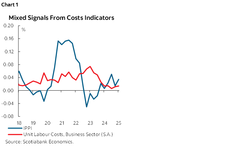
So, what does this imply for inflation and monetary policy going forward? The answer is far from straightforward, as there are many limitations to these individual measures. For instance, mapping IPPI to inflation is challenging because producer prices do not fully pass through to consumer prices. In fact, there is little empirical evidence that IPPI reliably forecasts CPI outside of the pandemic period; correlations between the two are largely contemporaneous. Similar caveats can apply to unit labour costs and wage indicators.

One thing is clear: no single cost metric can tell the full story. Identifying the “right” cost measure for inflation analysis is empirically complex. Firms face multiple cost pressures (wages, raw materials, intermediate inputs, import prices, energy) each with its own dynamics. Moreover, volatile costs can be absorbed by profit margins or offset elsewhere, meaning they may never translate into consumer prices.

AN UNDERLYING COST INDEX

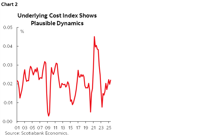
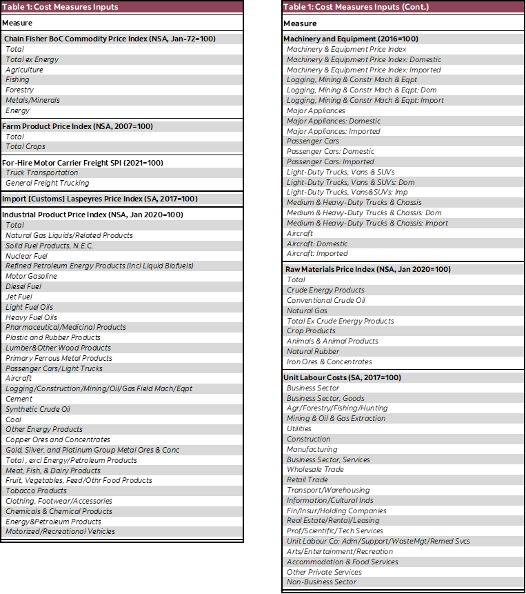
One way to address this issue of “dimensionality” is by constructing an underlying cost index (UCI). We do this using a standard factor model that summarizes information from a wide range of cost measures, including producer prices, unit labour costs, import prices, and commodity prices (see table 1 in the appendix for the complete list).¹

Factor models are well established in macroeconomic analysis and are commonly used to extract signals from large datasets. The idea is that while each cost series exhibits idiosyncratic fluctuations, there is an unobserved common factor influencing all of them. By isolating this factor, we aim to capture the broad cost-pressure signal and filter out indicator-specific noise. The resulting index, the UCI, reflects the common movement across cost indicators while removing idiosyncratic volatility. Conceptually, it serves as a “core” measure of costs, similar to the core inflation measures used by central banks to gauge underlying inflation.

Chart 2 shows the dynamics of this underlying cost measure over history.² Overall, the dynamics appear plausible: it declined sharply during the global financial crisis and rose rapidly during the 2021–22 inflation episode. More recently, cost pressures eased significantly in 2023 and have now recovered, sitting close to their historical average. While we see a recovery in the cost measure, it still contrasts with the recent strength in PPI. Historically, we find the index is closely correlated with commodity prices and the Canadian dollar, reflecting Canada’s exposure to global cost shocks. It is also correlated with the output gap, indicating that domestic demand generally influences costs as well.

LITTLE IMPLICATIONS FOR INFLATION DYNAMICS

Returning to our original question: what does this mean for inflation and the BoC’s policy decisions? We examine this from two angles: 1) its ability to explain inflation dynamics and 2) its role in shaping inflation risks.

To gauge the role of costs in inflation dynamics, we test whether our underlying cost index (UCI) adds explanatory power within a simple Phillips curve framework. In principle, if rising costs exert an influence on inflation that is not already captured by the business cycle (the output gap), then the UCI should materially improve model fit.

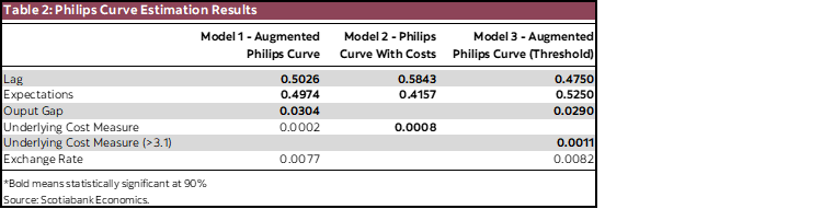
We begin with a standard Phillips curve of core inflation—including lagged inflation, the output gap, the exchange rate, and inflation expectations—and augment it with the UCI.³ The cost index enters with the expected positive sign, but the coefficient is not statistically significant. However, when we remove the output gap and the exchange rate and instead rely solely on the UCI, the coefficient becomes positive and statistically significant (see table 2 in appendix for estimation results). This indicates that while the UCI is clearly correlated with inflation, it does not add much information beyond what’s already embedded in traditional inflation drivers. From this perspective, the recent firming in cost measures should not materially alter the near-term inflation outlook.

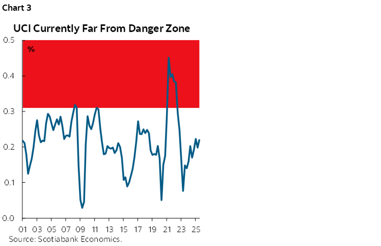
We do, however, find evidence of threshold effects. When cost growth exceeds roughly 3.1%, the relationship with inflation becomes statistically significant (chart 3). This pattern is intuitive: when cost pressures are modest, firms may hesitate to pass them through for fear of losing customers; but when costs rise sharply, firms are effectively forced to adjust prices. Importantly, these cost levels are rarely observed, and current readings sit comfortably below this danger zone.

THE CAUTIONARY TALE OF RISING COSTS

Our earlier results suggest that rising costs have limited implications for inflation once we account for cyclical conditions. But this does not mean they can be totally ignored. While costs may add little to the baseline inflation forecast, they can still play a material role in shaping inflation risks.

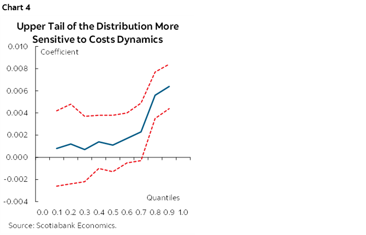
To assess this, we turn to a quantile version of the Phillips Curve. While standard regressions techniques focus on predicting average inflation outcomes, the Quantile Phillips Curve evaluates how drivers influence the full range of possible inflation outcomes. Put differently, it tells us whether a given variable shifts the tails of the distribution more than the centre, i.e. affecting the balance of risk.⁴ Technically, we use a direct forecast technique where we run quantiles regression of core inflation at time t+4 on a constant, contemporaneous inflation, the output gap, and the cost measure. Appendix 2 provides more technical details on quantile regressions and how they are used to assess macro risks.

Our estimates show that the upper quantiles of the inflation distribution react more strongly to changes in the cost measure than the middle quantiles. Chart 4 illustrates this clearly: coefficients rise steadily as we move into the upper tail. This implies that rising costs do not meaningfully move the median inflation forecast, consistent with our earlier results, but they do push up the right-hand tail of the distribution, increasing the probability of higher-than-expected inflation. In other words, costs act more as an amplifier of upside inflation risks than a steady driver of inflation itself. They increase the probability of bad outcomes.⁵

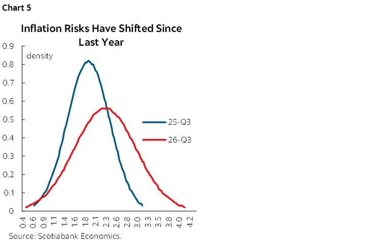
This distinction is particularly important in today’s environment. Cost pressures are recovering, creating conditions in which upside risks become more salient. As shown in chart 5, the predictive density for the 2026Q3 inflation has shifted notably compared with last year, while the median of the distribution has risen only modestly. The mass in the upper tail, especially above 3%, has increased significantly. In other words, the central forecast has barely budged, but the risk of an inflation surprise to the upside is meaningfully higher than it was a year ago.

MACRO AND POLICY IMPLICATIONS

Taken together, the analysis suggests that rising costs do not yet warrant a meaningful upward revision to the inflation forecast. Cost pressures have rebounded from recent lows but remain comfortably below levels historically associated with strong price pass‑through.

However, the risk environment has changed. Upside risks to inflation are more prevalent than a year ago and remain elevated relative to the pre‑pandemic period. This shift in the balance of risks carries important implications for the Bank of Canada; the increased likelihood of upside inflation surprises argues for a more cautious policy posture.

In our view, this reinforces the case that the Bank is unlikely to continue cutting rates in this cycle provided that nothing major happens on the tariff front depending upon their net effect on supply and demand, among other non-tariff risks. A neutral, or even slightly risk averse, stance appears more appropriate given the current configuration of cost pressures and the narrowing of economic slack.

¹ While these captures observed costs, it may not capture all costs firms are facing. A notable example would be that reorganizing supply chains and finding new clients in other markets may not be fully captured by the underlying data, and therefore in the cost index.

² The pure extracted factor is projected on inflation to get interpretable levels.

³ Core inflation is defined in this note as CPI excluding food and energy.

⁴ Quantile regressions have often been proposed by the literature to estimate predictive densities in a macro-risk context. In particular, see the seminal work by Adrian et al. (2019) on economic activity and Lopez-Salido and Loria (2024) for an application to US inflation. For a Canadian application on economic activity, see Duprey and Ueberfeldt (2020).

⁵ The coefficients on the output gap are not statistically significant in this framework.

APPENDIX 1

APPENDIX 2: QUANTILE REGRESSIONS AND MACRO RISKS

Standard OLS regression estimates the conditional mean of a dependent variable given a set of explanatory variables. In the context of inflation, an OLS Phillips curve describes how expected inflation evolves on average in response to some economic drivers. In contrast, quantile regression focuses on the relationship between conditional quantiles of inflation and economic drivers. So rather than focusing on the mean, it allows the relationship between inflation and drivers to differ across the distribution of inflation.

where τ denotes the quantile of interest (e.g., τ = 0.5 for the median, τ = 0.9 for the 90th percentile, etc.).⁶

In practice, quantile regressions are estimated separately for each quantile of interest. So, we estimate one Phillips curve for the lower tail (τ = 0.1), the median (τ = 0.5), the upper tail (τ = 0.9), etc. The resulting set of coefficients can be interpreted as the relationship between inflation and its drivers across these quantiles. When a coefficient rises monotonically with τ, as is the case with the UCI, it indicates that the variable affects upside inflation risks rather than the central tendency.

Once we have these estimates, we can use the equation above to project the quantiles and obtain their fitted values over history. We then get levels of predicted quantiles at each point in time, therefore revealing how risks dynamics have evolved. Finally, these predicted values for each quantiles can be fitted on a distribution to produce densities (like in chart 5). In the context of this note, we use a Student’s t distribution.

⁶ For more details on the quantile regression methodology, see Koenker (2005). In practice, quantile regressions techniques are available in standard econometrics packages.